Background
SlowMoMan ("SLOW MOtions on MANifolds") is an open-source tool for helping biologists (and data practitioners in general) better understand their embeddings. Read on for a deeper dive into the methodology behind the app. Scroll past that if you want to get your hands dirty with a real use case!
Methodology
SlowMoMan proposes a novel way for users to analyze embeddings. In particular,
the app works by
- Let the user draw a path anywhere along the embedding
- Along the path, sample 512 evenly spaced points (the number of points is controlled by the "Number of bins" parameter)
- For each of the 512 points, find the nearest neighbour in the actual 2D embedding
- For each of the nearest neighbours found, we grab its respective vector from the original feature space
- This ordered list of vectors from the original space is then analyzed via the FFT metric or the autocorrelation metric. The metrics serve as a way to rank or sort each of the features in the original space by their potential "significance". More "significant" features are ranked higher (of course, the meaning of "significance" will vary depending on the metric used!).
Guided Use Case
In order to use SlowMoMan we'll need two CSV files:
Secondly, the CSV containing the high dimensional data should contain all the features you want to analyze. Note, if you accidentally include an "index" column (ie., a column of 1-2-3-4...), that will be used in the analysis by SlowMoMan, but it won't affect the results of the other features (so you can safely ignore this column in the results output).
To follow along, download the QuickStart data from the SlowMoMan Google Drive folder: https://drive.google.com/drive/folders/1FZf2SqQ55KBu7iaIj1r1qqNUX8il6mJQ?usp=sharing
In this example, we use data obtained by Zeisel et al. (2015). The original dataset has 2180 features, each of them representing a gene. There are 2816 rows, each corresponding to a single cell from the mouse brain. Each of the cells in this dataset belong to 1 of 7 subclasses of brain cell (interneurons, pyramidal SS, pyramidal CA1, oligodendrocytes, microglia, endothelial-mural, astrocytes_ependymal). From this large dataset, we run t-SNE to obtain a 2D embedding of the original data. Finally, we have all we need to begin using SlowMoMan!
Step 1: Upload Datasets
Here we will simply upload our 2D embedding (with the "X", "Y", and "class" columns) and our original feature space.

Step 2: Draw Path
Next you can draw a path by hovering over a point and dragging. Since the nearest neighbour algorithm will hunt for points closest to your line, try to draw directly over points you want to capture.

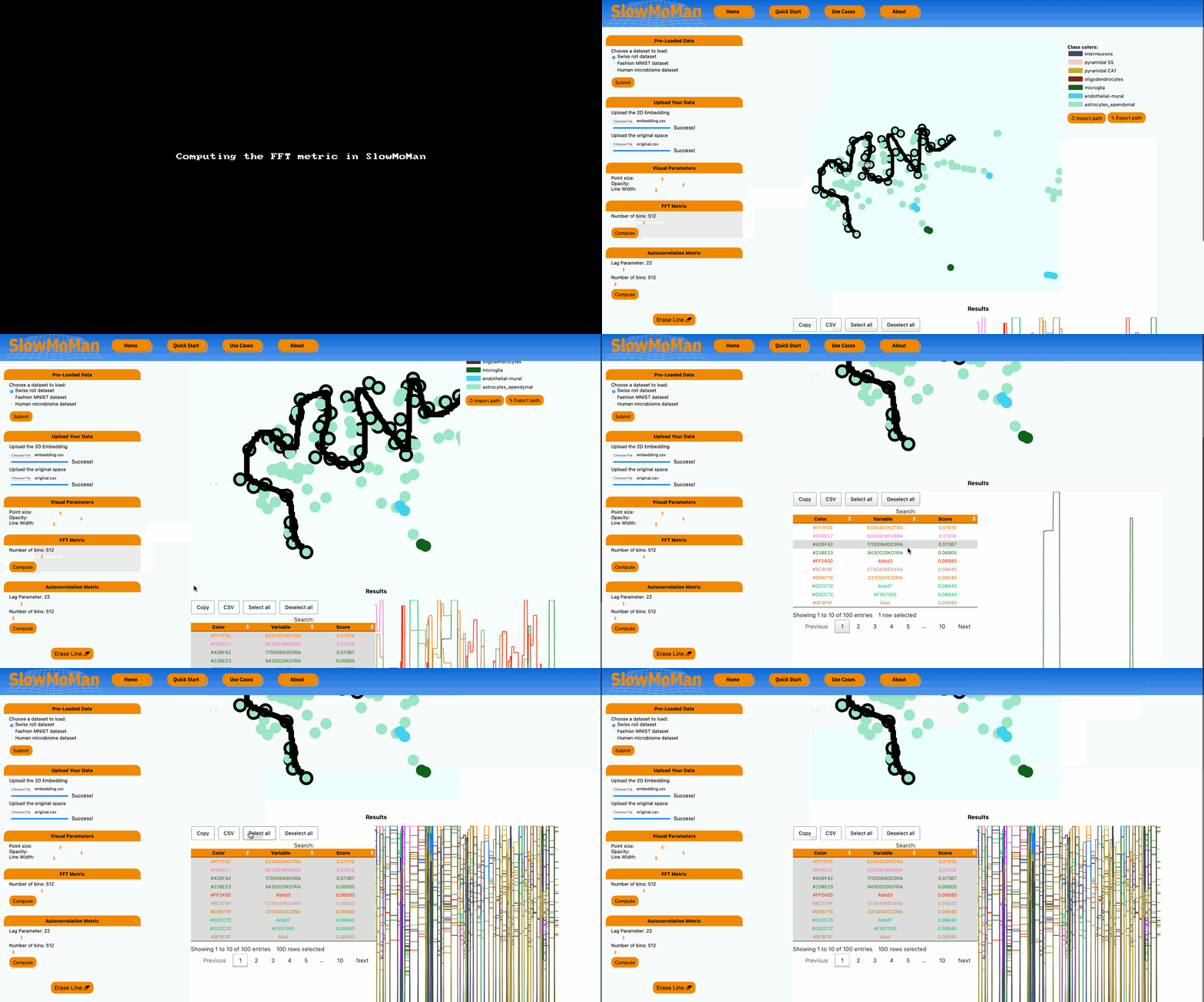
Step 3: Compute FFT and Save Results
Once you've drawn a line you can choose between computing the FFT metric or the autocorrelation metric. Recall that "Number of bins" is the number of points we will sample from your line (e.g., with 512 bins, we sample 512 evenly spaced points across your line, and for each of those 512 points we'll find their nearest neighbour in the embedding space).
Notice that after you submit, the points captured by the nearest neighbour algorithm are outlined in black. These are the points that are used in the final computation, so feel free to redo the path and play around until you get the path you want. Note that the nearest neighbour computation is done via a quad tree and may not yield perfect results!
In the results section below, you can see how the values of each feature changes along your path. Click on each feature one-by-one and feel free to zoom in to really understand how that particular features behaves along your path. You can also save your results by clicking "Select All" and then "CSV" to download a CSV of your scores.

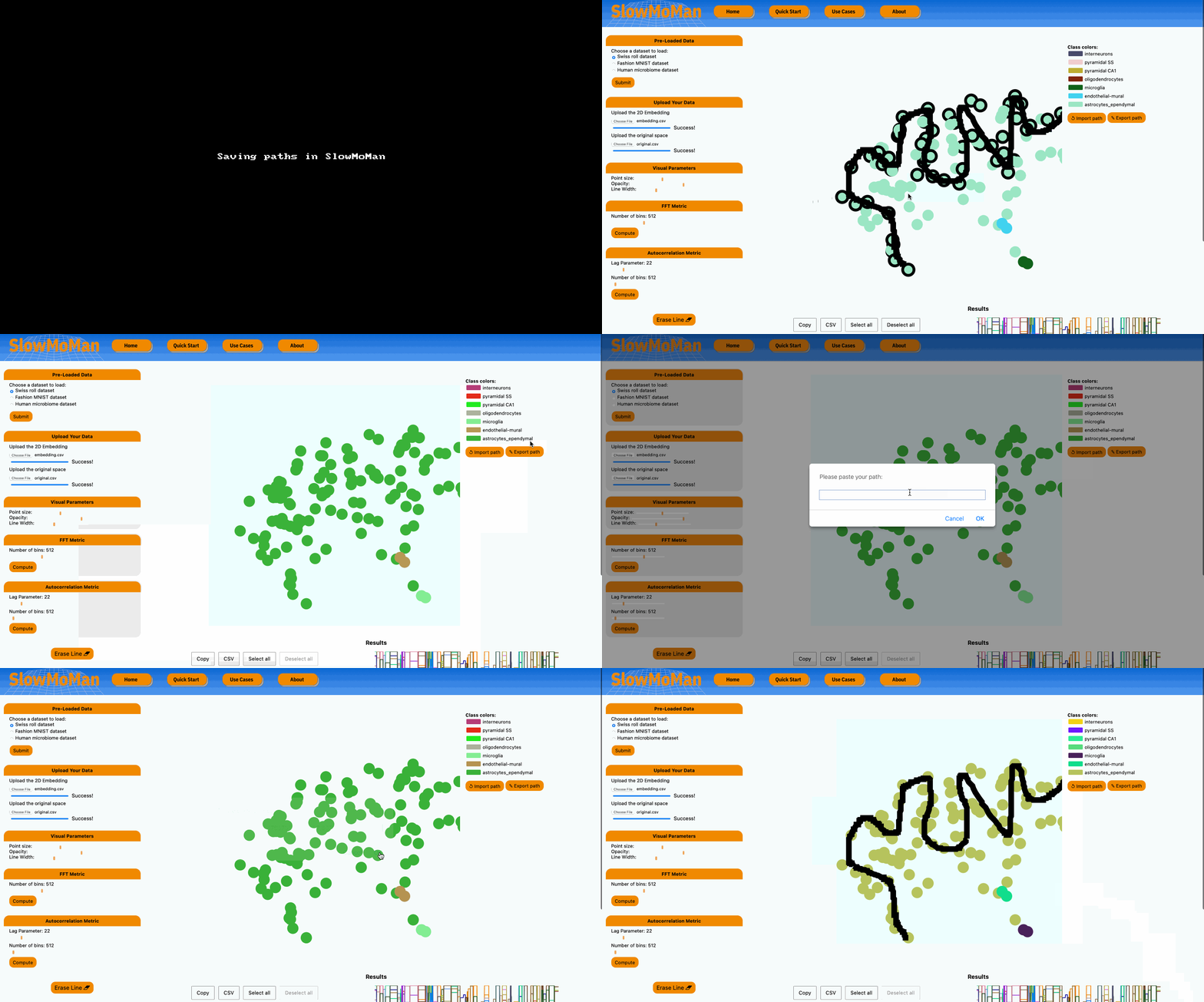
Step 4: Save and Share Path
If you end up with results you want to replicate, you need to save your path. To do so, hit "Export Path" and it will be copied to your clipboard. From there, you can paste this into a .txt file or any document. When you need to import a path, simply copy it from wherever you saved it, click "Import Path" and paste it into the prompt.

- A high dimensional dataset (call this HD data)
- A 2D embedding of that dataset (call this 2D data)
Secondly, the CSV containing the high dimensional data should contain all the features you want to analyze. Note, if you accidentally include an "index" column (ie., a column of 1-2-3-4...), that will be used in the analysis by SlowMoMan, but it won't affect the results of the other features (so you can safely ignore this column in the results output).
To follow along, download the QuickStart data from the SlowMoMan Google Drive folder: https://drive.google.com/drive/folders/1FZf2SqQ55KBu7iaIj1r1qqNUX8il6mJQ?usp=sharing
In this example, we use data obtained by Zeisel et al. (2015). The original dataset has 2180 features, each of them representing a gene. There are 2816 rows, each corresponding to a single cell from the mouse brain. Each of the cells in this dataset belong to 1 of 7 subclasses of brain cell (interneurons, pyramidal SS, pyramidal CA1, oligodendrocytes, microglia, endothelial-mural, astrocytes_ependymal). From this large dataset, we run t-SNE to obtain a 2D embedding of the original data. Finally, we have all we need to begin using SlowMoMan!
Step 1: Upload Datasets
Here we will simply upload our 2D embedding (with the "X", "Y", and "class" columns) and our original feature space.

Step 2: Draw Path
Next you can draw a path by hovering over a point and dragging. Since the nearest neighbour algorithm will hunt for points closest to your line, try to draw directly over points you want to capture.

Step 3: Compute FFT and Save Results
Once you've drawn a line you can choose between computing the FFT metric or the autocorrelation metric. Recall that "Number of bins" is the number of points we will sample from your line (e.g., with 512 bins, we sample 512 evenly spaced points across your line, and for each of those 512 points we'll find their nearest neighbour in the embedding space).
Notice that after you submit, the points captured by the nearest neighbour algorithm are outlined in black. These are the points that are used in the final computation, so feel free to redo the path and play around until you get the path you want. Note that the nearest neighbour computation is done via a quad tree and may not yield perfect results!
In the results section below, you can see how the values of each feature changes along your path. Click on each feature one-by-one and feel free to zoom in to really understand how that particular features behaves along your path. You can also save your results by clicking "Select All" and then "CSV" to download a CSV of your scores.

Step 4: Save and Share Path
If you end up with results you want to replicate, you need to save your path. To do so, hit "Export Path" and it will be copied to your clipboard. From there, you can paste this into a .txt file or any document. When you need to import a path, simply copy it from wherever you saved it, click "Import Path" and paste it into the prompt.

